6: Address Translation
Address Translation Concept
From virtual address to physical address.
Memory protection(内存保护)
地址转换允许操作系统为每个进程分配独立的虚拟地址空间。这样,一个进程无法访问或修改其他进程的内存区域,从而防止恶意或错误的访问,提升系统安全性。Memory sharing(内存共享)
通过地址转换,多个进程可以安全地共享某些物理内存区域(如共享库或数据),而不会影响各自的私有数据。操作系统可灵活地将同一物理页映射到不同进程的虚拟地址空间。Flexible memory placement(灵活的内存放置)
地址转换使得虚拟地址与物理地址解耦,操作系统可以将进程的内存分散地放置在物理内存的任意位置,而不要求连续分配,提高了内存利用率和碎片管理能力。Sparse addresses(稀疏地址空间)
虚拟地址空间可以远大于实际物理内存,允许进程分配大但稀疏的地址空间。只有实际用到的部分才会分配物理内存,节省资源并支持大数据集或内存映射文件。Runtime lookup efficiency(运行时查找效率)
地址转换机制(如页表和 TLB)设计为高效,能在每次内存访问时快速完成虚拟地址到物理地址的映射,保证程序运行速度不会因转换过程显著降低。Compact translation tables(紧凑的转换表)
地址转换表(如多级页表)结构设计紧凑,既能支持大地址空间,又能节省内存开销,避免为未使用的虚拟地址分配过多资源。Portability(可移植性)
虚拟地址空间让程序无需关心物理内存布局,提升了软件的可移植性。程序可以在不同硬件或操作系统上运行,而无需修改内存访问逻辑。
- When translation exists, processor uses virtual addresses, physical memory uses physical addresses
- Not every processor/OS has address translation, e.g., certain embedded chips
- Address translation involves intensive hardware-OS cooperation
- Address space: all the addresses and state a process can touch
- Each process and kernel has different address space
Segmentation
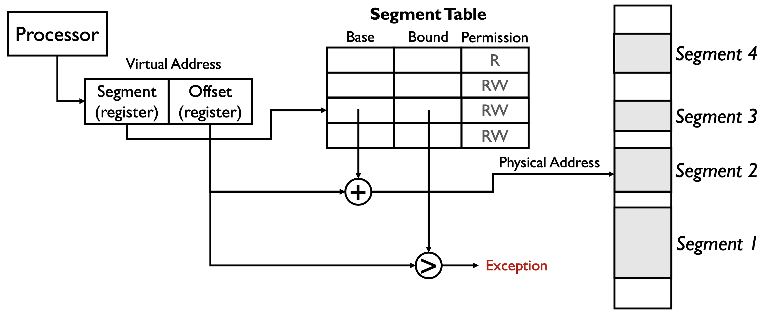
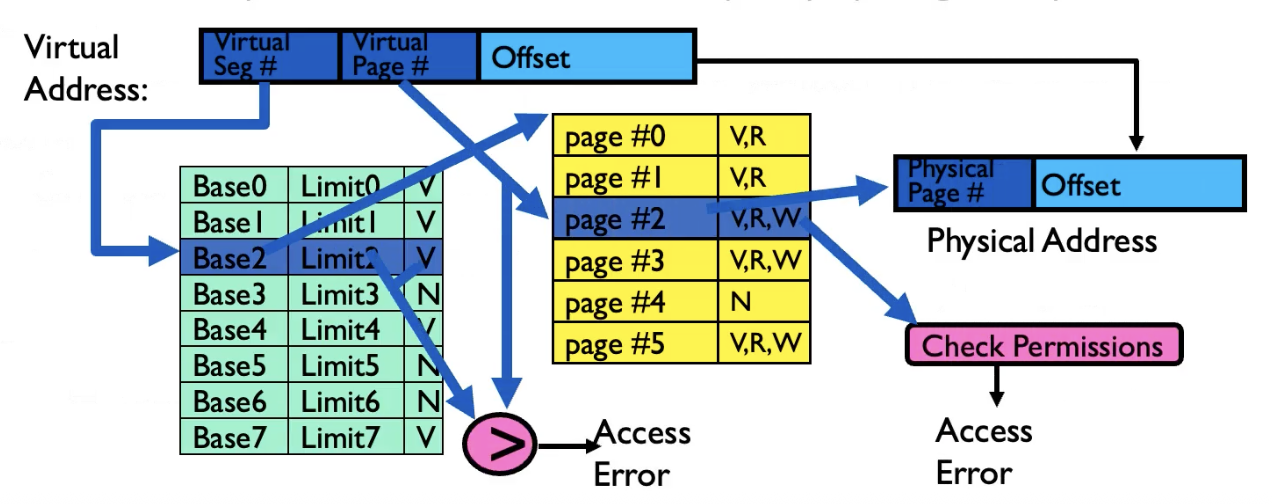
在这一页的分段存储(Segmented Memory)图示中,virtual address(虚拟地址)的结构由两部分组成:
- Segment(段寄存器):用于选择当前访问的是哪一个段(segment),即在分段表中查找对应的条目。
- Offset(偏移寄存器):表示在该段内的偏移量,即访问该段内的具体位置。
虚拟地址结构可以用如下形式表示: \[ \text{Virtual Address} = (\text{Segment}, \text{Offset}) \]
图中的 “+” 和 “>” 的意义如下:
- “+”:表示将分段表中查到的该段的 Base(基址)与 Offset(偏移量)相加,得到物理地址。 \[ \text{Physical Address} = \text{Base} + \text{Offset} \]
- “>”:表示将 Offset 与 Bound(界限)进行比较。如果 Offset 超过 Bound,说明访问越界,触发 Exception(异常)。
简要流程:
- 处理器根据虚拟地址中的 Segment 字段查找分段表,获得该段的 Base、Bound 和权限。
- 检查 Offset 是否小于 Bound(“>”比较),否则异常。
- 用 Base + Offset(“+”运算)得到物理地址,完成地址转换。
这样设计既实现了内存保护,也支持灵活的内存分布和访问控制。
可以看到 Figure 1 最右边的 physical memory 中有许多 holes,为什么会形成这些 holes?如果一个 process branches into these holes 会发生什么?
- 为什么物理内存会有 holes(空洞)(Why we abandon segmentation)
- 动态分配/释放:进程创建、退出或调整段/页大小后,物理上被释放的区域会留下不连续的空闲区(外部碎片)。
- 不同大小/对齐:段大小各异且要求对齐,会产生不能被当前需求填满的空闲间隙。
- 内核/设备保留:内核空间、设备映射等也占用物理地址区间,形成不可用的间隔。
- 若只用段式分配(不做压缩/搬迁),这些空洞会累积。
- 动态分配/释放:进程创建、退出或调整段/页大小后,物理上被释放的区域会留下不连续的空闲区(外部碎片)。
- 如果进程“branch into these holes”(跳转或访问到这些空洞)会发生什么
- 若虚拟地址没有被映射到有效段/页:MMU/段表检测到无效映射或权限不符,CPU 产生异常(segmentation fault / protection fault)。操作系统通常终止该进程或发信号(如 Unix 的 SIGSEGV)。
- 在按需分页系统中:若虚拟地址在合法的地址空间但对应页面尚未驻留,首次访问会触发 page fault,操作系统可以分配物理页并完成映射(例如分配零页或从磁盘加载),然后继续执行。
- 在分段模型中:若 offset >= bound,会立即触发段越界异常;若 offset < bound 但权限不够(如试图写入只读段),会触发保护异常。
- 简言之:未映射或越界访问不会“读到随机数据”,而是由硬件/OS 捕获并处理(异常、分配页面或终止进程)。
- 若虚拟地址没有被映射到有效段/页:MMU/段表检测到无效映射或权限不符,CPU 产生异常(segmentation fault / protection fault)。操作系统通常终止该进程或发信号(如 Unix 的 SIGSEGV)。
- 操作系统的应对
- 使用分页或段页结合以减轻外部碎片;采用内存压缩/搬迁(compaction)或交换(swap)来回收连续空间。
- 在允许情况下使用按需分配,首次访问时由 OS 分配并初始化物理页面。
- 使用分页或段页结合以减轻外部碎片;采用内存压缩/搬迁(compaction)或交换(swap)来回收连续空间。
结论:holes 是物理上未分配的空闲区,直接跳到这些区域通常会引起硬件异常或页面缺失,需由 OS 通过映射/分配或强制终止来处理。
分段存储(Segmented Memory)在实际操作系统中的实现方式存在较大差异:
- 某些操作系统(如 Multics)会为每个数据结构分配一个段,以实现细粒度的保护和进程间共享。
- 而大多数现代系统只用分段机制来管理粗粒度的内存区域(如代码段、数据段等),不再为每个小对象单独分段。
The power of segmentation
- access control
- code sharing (library routine)
- inter-process communication
- efficient management of dynamically allocated memory
Each process has its own segment table
The principle downside of segmentation: overhead of managing a large number of variable size and dynamically growing memory segments
- external fragmentation: free space becomes noncontiguous
- compacting the memory is very slow
- it becomes even more complex if the segments can grow (like heap)
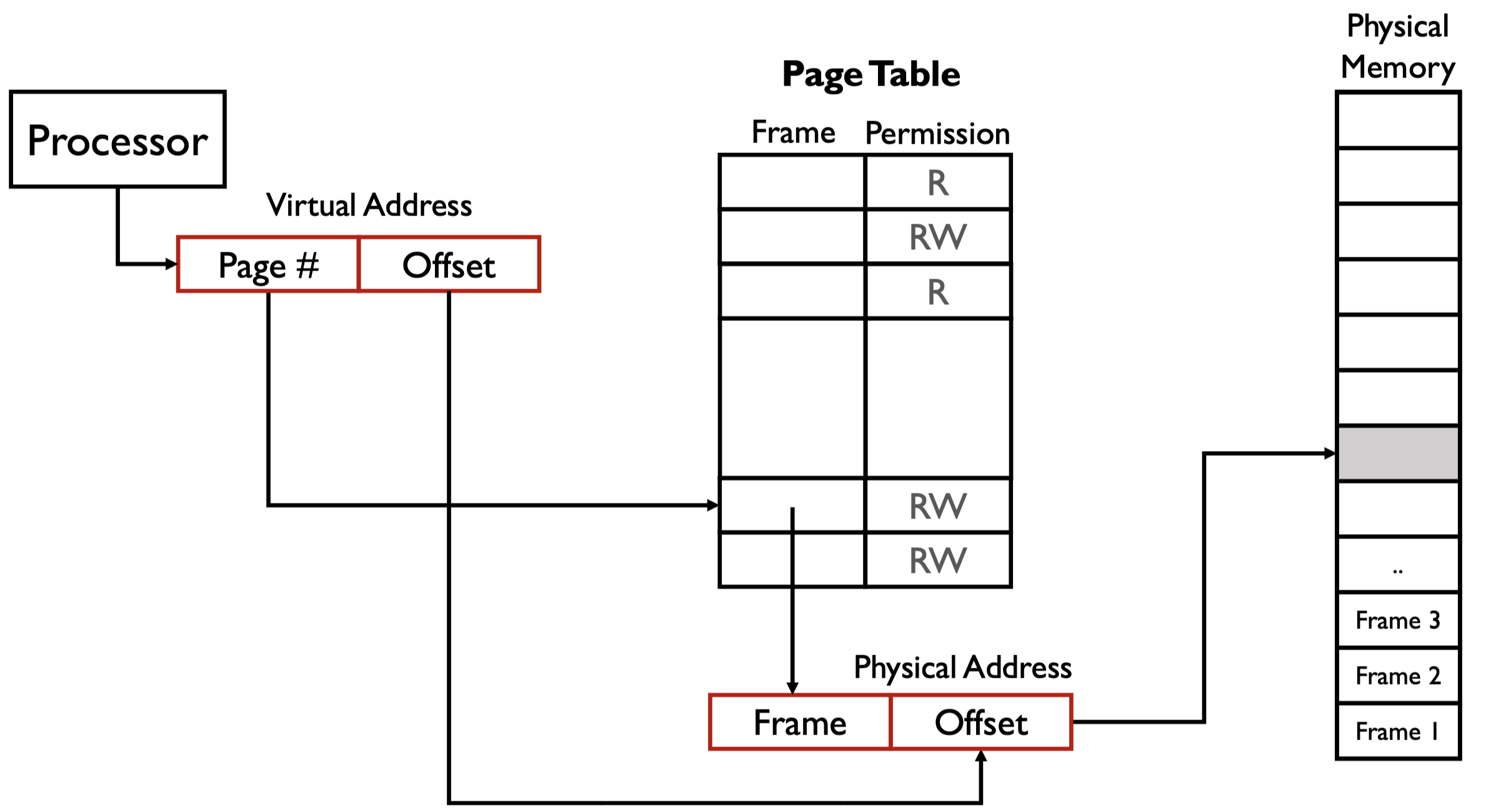
Paging
Def. Paging: allocate memory in fixed-sized chunks called page frames.
A page table stores for each process whose entries contain pointers to the page frames.
- More compact than segment table because it does not need to store “bound”
Memory allocation becomes very simple: find a page frame.
Single-Level Paging
单级页表虽然解决了很多问题(如支持页面共享),但页表本身可能非常大,甚至超过进程实际使用的内存。
- 对于大地址空间,每个进程都需要分配完整的页表,即使实际只用到很少的页面。
- 这会导致大量内存浪费,尤其是进程数量多或每个进程实际用到的页面很少时。
页内偏移 offset 由页的大小决定,我们应该设计一个能恰好访问整个页的 offset。
page table 是一个数组,基于下标访问,也就是说,一旦创建,必定占用一定大小的内存空间。
在 Figure 2 中,假设页的大小为 \(4 \ \text{KB}\),所以我们需要能映射范围最大为 \(2^{12}\) 的 offset。
在 Figure 2 中,我们设计的分页,一个进程能访问的最大虚拟地址为 \(2^{32} - 1\),但实际能访问的物理地址也是 \(2^{32} - 1\),这是因为 page table 中的 frame 也是 \(20\) 位。
整个 page table 的大小为,\(2^{20} \times 4 \ \text{bytes} = 4 \ \text{MB}\)。这个数值大吗?需要注意的是,每一个进程都有一个大小为 \(4 \ \text{MB}\) 的 page table,进程过多会占用巨大内存。这也引出了一个问题,实际上一个进程大概率用不完 \(4 \ \text{MB}\) 大小的 page table,从而导致浪费
Multi-level Paging
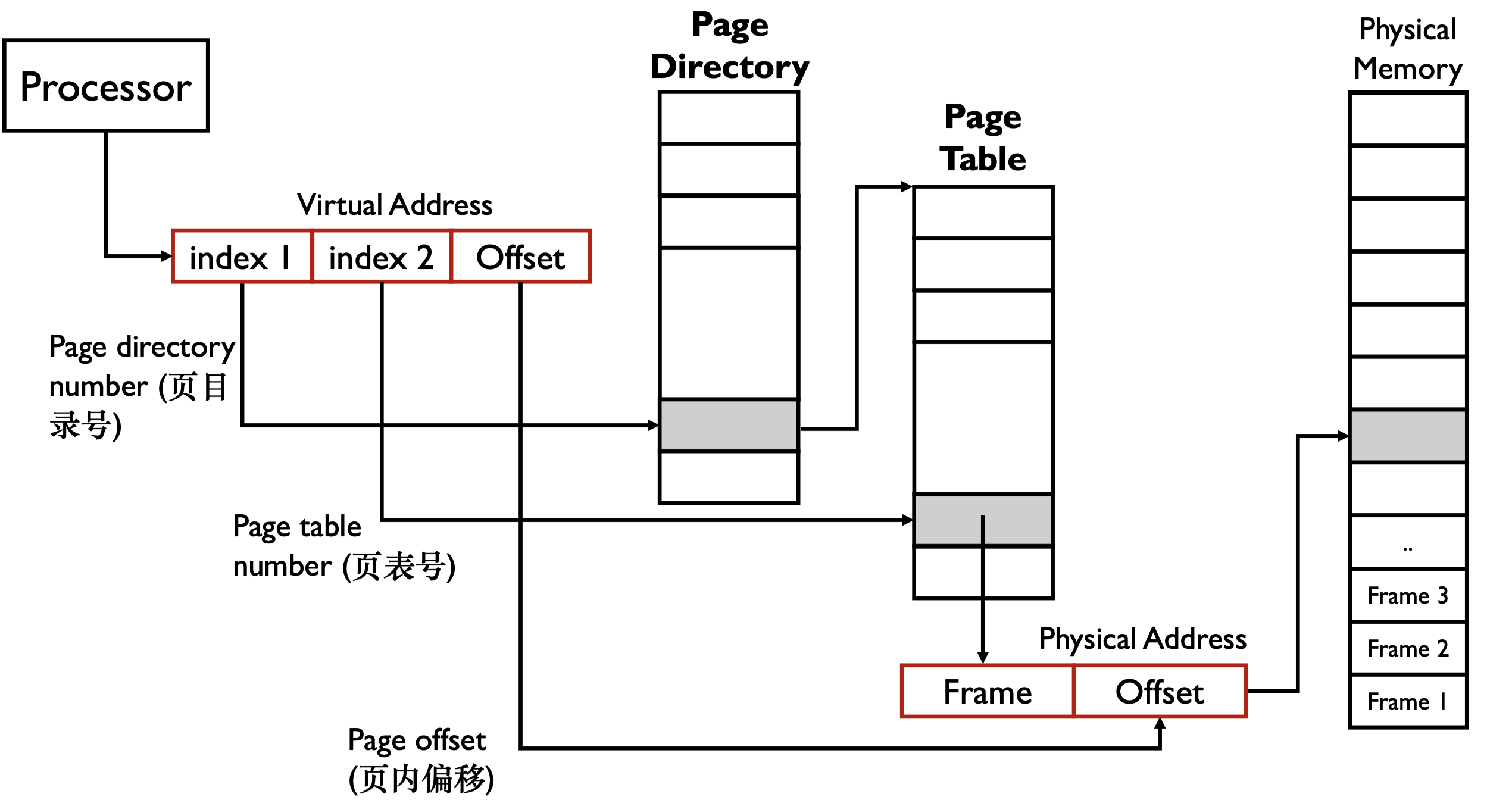
假设 index 都是 \(10 \ \text{bits}\),则此时一个 page table 大小好为 \(2^{10} \times 4 \ \text{bytes} = 4 \ \text{KB}\)
x86 中有一个寄存器,
CR3,指向 page directory 的起始地址。进程与进程之间进行切换时只需要切换CR3即可。CR3保存在 PCB 中。假设一个进程只用到 \(1 \ \text{KB}\) 的内存,对一级页表,需要 \(4 \ \text{MB}\) 的内存,对多级页表需要 \(8 \ \text{KB}\) 的内存。
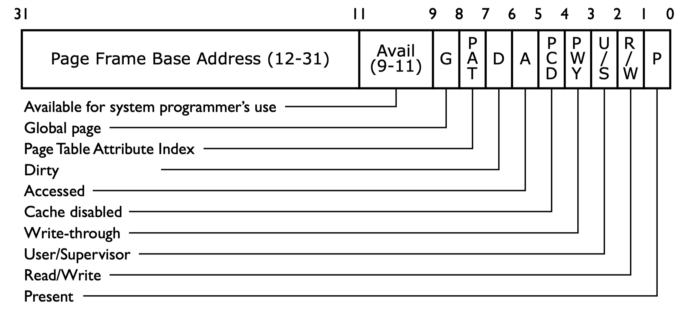
Page Directory Entry
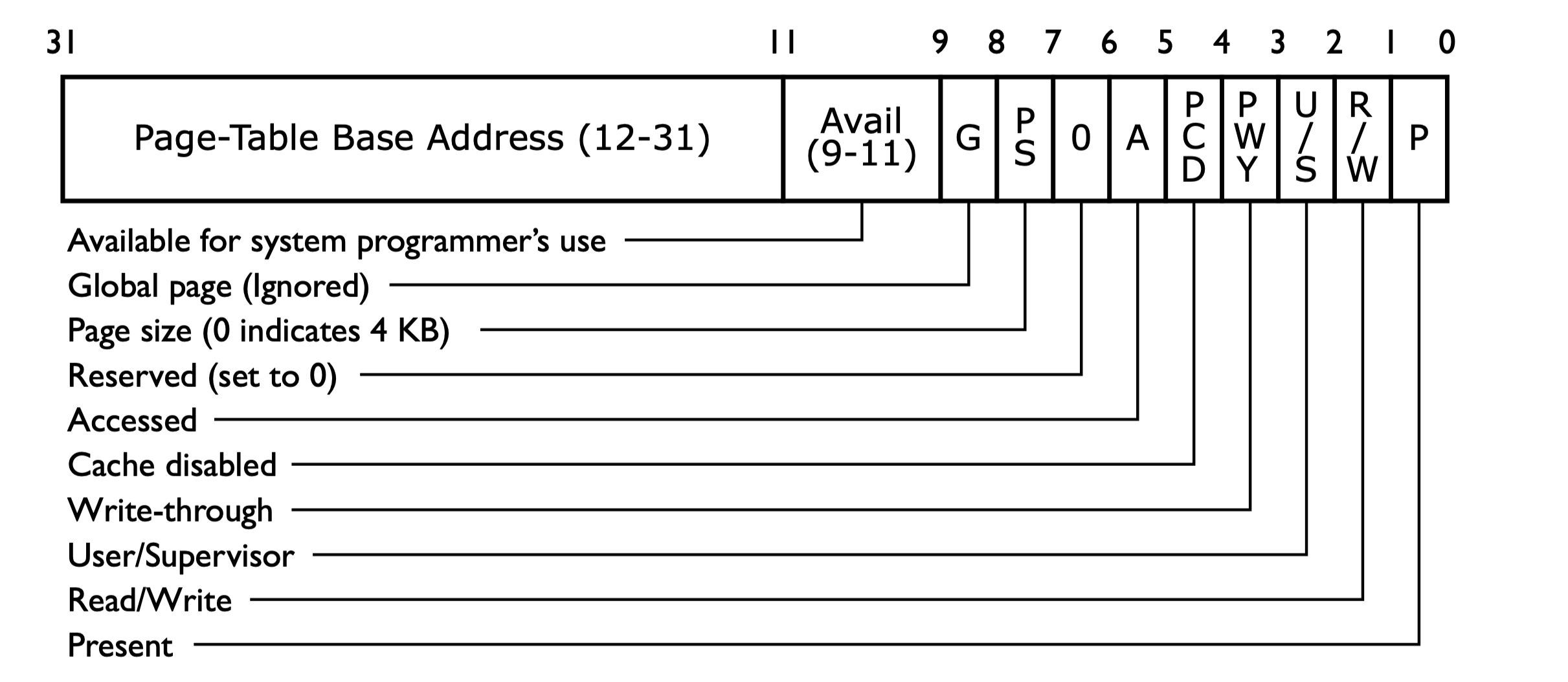
Page Table Entry
Memory Management Unit
Def. Memory Management Unit (MMU): the hardware that actually does the translation, usually located in CPU.
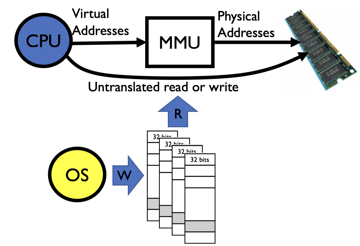
MMU 会与
CR3寄存器相连。映射的关系是由操作系统决定的,也就是操作系统填入 MMU,但这个映射过程是由硬件完成的,效率会更高。
Page size shall be neither too small or too large
- too small: large page table sizes; low cache hit ratio
- too large: memory waste
- typical range: \(512 \ \text{B}\) to \(8192 \ \text{B}\); default \(4 \ \text{KB}\) on Linux
Each process has their own page table
- the same address of different processes translate to different physical locations, unless the page is shared
Pages tables can be sparse, because not every PDE has a corresponding page table.
Page Fault
- Page Fault(缺页中断 exception):当 CPU/MMU 访问的虚拟地址没有被映射到物理内存时发生。
- 软缺页(Pure/Soft):如页面被换出或共享页未驻留,操作系统处理后可继续访问。
- 硬缺页(Invalid/Hard):如写入只读页、访问未分配页等,通常导致段错误(Segmentation fault)。
- 现代操作系统中的
malloc行为:malloc只分配虚拟地址空间,不会立即分配物理内存。- 只有当程序真正访问这块内存时,才通过缺页中断分配物理页。
- 这样做可以节省物理内存,提高资源利用率。
x86 Multi-Level Paging
- Why PDE/PTE uses \(20\) bits for addressing the next-level table or page?
- page directory/tables are always page-aligned (\(\% 4 \ \text{K} = 0\))
- What needs to be switched on a context switch?
- the page directory, stored in
CR3
- the page directory, stored in
- If a process needs \(1\) page for its data, how many it will actual take?
- \(3\) in total (\(1\) page directory, \(1\) page table, \(1\) page for its data)
- The largest address can be accessed in 2-level paging (\(32\) bits address)?
- \(2^{10} \times 2^{10} \times 4 \ \text{K} = 4 \ \text{G}\)
CR3stores the virtual or physical address of the page directory?- physical address
- How about the PDE/PTE?
- physical address
- How can kernel manipulate the page directory/tables?
- e.g., getting the physical address of a given virtual address?
- 想得到
a : b : c这个虚拟地址的物理地址 - 我们可以得到的
CR3寄存器的物理地址 - 新建一个虚拟地址,将其指向的页目录映射到
CR3,也就是自映射;将其指向的页表项指向a,偏移设置为c - 我们对新虚拟地址取值,值是原先虚拟地址的对应页表的值,也就是 page frame 这个物理地址一部分,将其与
c拼接,得到真正的物理地址
- 想得到
- e.g., getting the physical address of a given virtual address?
Pros
- Only need to allocate as many page table entries as we need for application
- in other words, sparse address spaces are easy
- Easy memory allocation
- Easy sharing
Cons
- One pointer per page (typically \(4 \ \text{K}\) - \(16 \ \text{K}\) pages today)
- Page tables need to be contiguous
- however, previous example keeps tables to exactly one page in size
- Two (or more, if \(> 2\) levels) lookups per reference
- seems very expensive
Paging with Segments
What about a tree of tables?
- lowest level page table \(\Rightarrow\) memory still allocated with bitmap
- higher levels often segmented
Copy-on-Write
How to implement an efficient fork()?
- Do not copy all contents immediately, but mark the pages/segment tables of both child and parent processes as “read only”
- When a write (from either child or parent) happens, it traps into kernel through page fault, and a private page is copied
A fork() followed immediately by a exec(), how many pages are really copied?
Page Coloring
Page Coloring or Cache Coloring technique helps reduce the cache miss in an app.
Consider two consecutive pages used by an application:
- their virtual set number must be different
- but their physical set number could be the same after translation (when the OS maps them to the physical pages whose page numbers have the sam last \(2 \ \text{bits}\)). In such a case, two addresses with the same offset within these two pages will in contention for the cache set

Solutions
- coloring the physical pages with the cache sets
- maps the application pages to as many colors as possible (so less contention)
Page coloring only works for L2/L3, not L1. Page coloring does not work for full associative cache.
Working Set
Def. Working Set; the memory needed by a program at a period
- could change at different phases
- better fit them into fast storage, e.g., L1 cache
Zipf Model
Def. Zipf Model: the frequency of visit to the k-th most popular page \(\propto \frac{1}{k^{\alpha}}\), where \(1 \leq \alpha \leq 2\).
Split L1 Cache
L1 cache often has two cache hardware: icache and dcache.
L2 and L3 are often one unified cache.
- L1 是从虚拟地址到物理地址,虚拟地址可以区分指令和数据;L2 和 L3 中的物理地址无法区分